blog-page - Cloud Engineer

Cloud Engineer

mailsforsahan@gmail.com

Call Me!

Big Data Analytics

Harnessing Big Data Analytics: A Deep Dive into Data Analysis and Imputation Techniques

In the evolving landscape of Big Data, the use of sophisticated analytics and imputation methods to manage and interpret vast datasets has become paramount. This blog post delves into the innovative approaches and technologies leveraged in the field of Big Data analytics, focusing on data analysis and the management of missing data, as demonstrated through a comprehensive case study of the billionaires.csv dataset.

01 – Understanding the Dataset

The billionaires.csv dataset serves as a rich repository of information on the world’s wealthiest individuals, detailing their demographics, company affiliations, and wealth sources. With 2,614 entries and 22 columns, this dataset offers a panoramic view of global wealth distribution and the economic sectors that propel it. The dataset not only tracks the financial status of these individuals but also explores various demographic factors such as gender and age, providing insights into the dynamics of wealth accumulation.

02 – Data Pre-Processing and Imputation

One of the critical steps in Big Data analytics is data pre-processing, which involves preparing the raw data for further analysis by cleaning and structuring it. In this case, the data pre-processing involved several key steps:

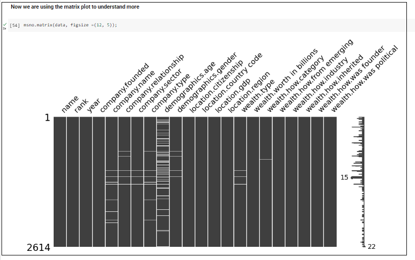
Handling Missing Values: The missingno library was utilized to visualize and address missing values within the dataset. Techniques such as matrix visualization helped identify the absence of data in crucial columns like company name, sector, and demographics.
Imputation Techniques: For numerical data like age, where zero values were inappropriate, these were replaced with the mean age to maintain data integrity. Similarly, missing categorical data, such as gender, were filled with ‘Not Given’, respecting the sensitivity and privacy of the data subjects.
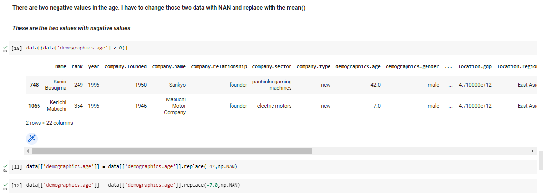
Data Cleaning: Negative values detected in the age column were corrected by converting them to NaN and then imputing them with mean values, ensuring the dataset’s accuracy and reliability.

These meticulous steps in data pre-processing underscore the importance of clean and precise data in analytics, as they significantly influence the outcomes of any subsequent analyses.

03 – Advanced Data Analysis

Post data cleaning, the analysis shifted towards extracting meaningful insights from the processed data. Using tools like Python, Pandas, and Jupyter Notebook, various analyses were performed, including:

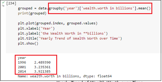
Wealth and Demographics: Analysis of the correlation between wealth and factors like age and gender, using statistical significance testing to validate hypotheses.
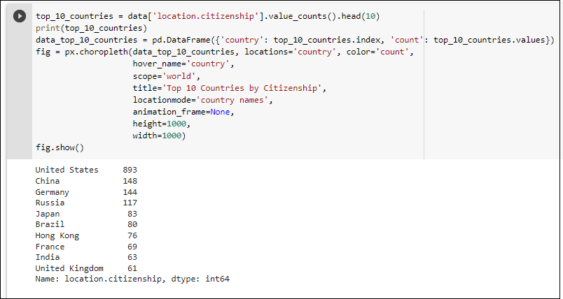
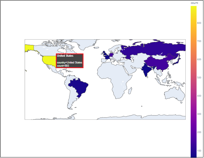
Geographical Insights: Identification of the top 10 countries with the highest number of billionaires, providing a geographical perspective on wealth distribution.
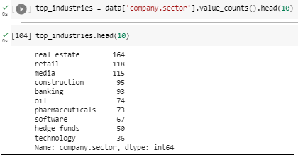
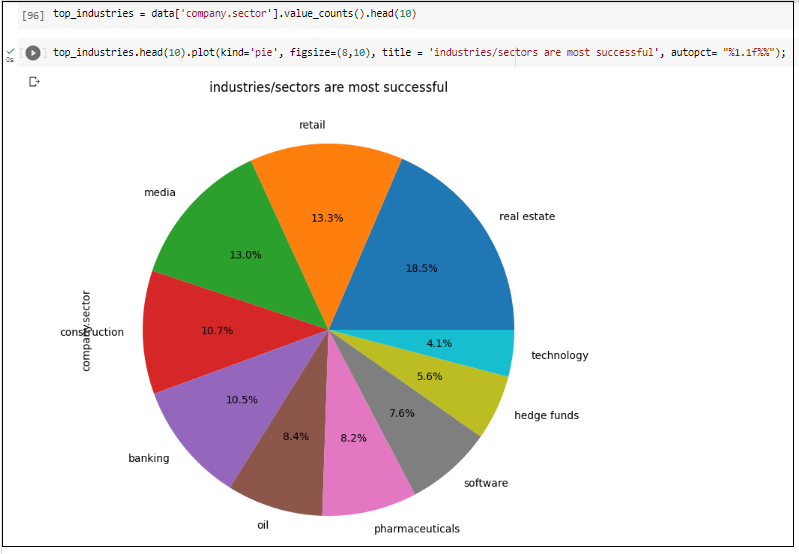
Sector Success: Examination of the most successful industries, highlighting sectors like technology and healthcare, which are predominant among the wealthiest individuals.

04 – Data pre-processing

By analyzing the dataset, there are a number of missing values and numerical numbers that are not appropriate with the column name. Here, in the below image, the missingno library is used to analyze the missing values visually. To identify more clearly, according to Figure 05, matrix visualization in the missingno library was used. According to the below diagram, the total row count is 2614 and there are missing values in company.name, company.relationship, company.sector, company.type, demographics.gender, wealth.type, wealth.how.category, wealth.how.industry.

Step 01 – Analyze the dataset and filter 0 values in the dataset.

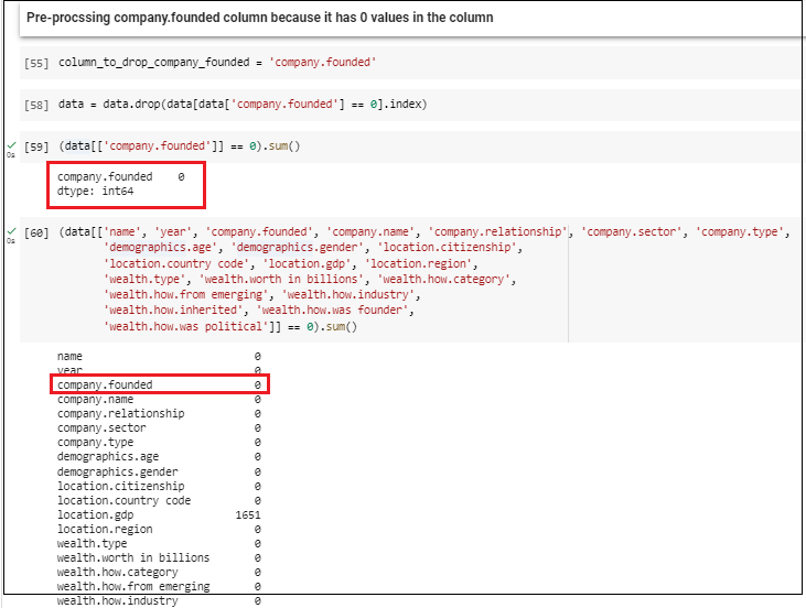
According to the dataset, below image demonstrates, the columns that contain 0 values. Out of all the columns, company.founded and demographics.age columns have 0 values which are not appropriate. Then the next step is to pre-process the demography.age column to have an accurate output.

Step 02 – Replaced 0 values with the mean of the demographic age column.

In the next step, replacing 0 values with NAN, and then, the replaced NAN values will be changed with the mean of the demographic.age column

Step 03 – Analyze whether the demographic.age column has any negative values.

After analyzing the dataset, there were two rows with negative values of demographic age. The first one is -47.0 and -7.0 which is not accurate, here, the negative values are converted to NAN values and then the NAN values are imputed by the mean of the column.

Step 04 – pre-process company founded column according to the below figure, there are 40 fields with 0 values in the company.founded column. When pre-processing company.founded column, the appropriate method is to use mean or any other method to guess the founded date and dropped the data which contains 0

Step 05 – pre-processing demographic.gender column.

According to Figure 12, there are 21 missing values in the demographic.gender column. For the pre-processing, the best method was to replace null values with ‘Not Given’ and the reason for making null values in the demographic.gender column is because people may refuse to specify their gender identity depending on personal factors.

Step 07 – Pre-processing company.relationship, company.sector column, company.type column and wealth. Type and once all the columns are pre-processed there are no null values in the data set

05 –What are the top 10 countries with the highest number of billionaires?

Here, a new variable was made as top_10_countries and used the location.citizenship column to select which column data is needed and finally, use value_counts() and head(10) to show the top 10 figures.

06 – Top 10 countries with geo map locations

05 –What industries/sectors are most successful?

When sorting the top industries in the dataset, a new variable was created name top_industries and selected company.sector column with value_counts() and sorted top 10 sectors.

06 –What are the main industries with the highest number of women billionaires?

When sorting the main industries with the highest number of women billionaires, demographics.gender is grouped with company sector. Then, to visualize the top industries, value_counts() with head(10) query was used.

07 –Trend of wealth worth over the time period

According to the dataset, wealth worth over time has significantly increased from 1996 onwards. The data was generated by, grouping year with wealth.worth in billions with the mean.

Conclusion and Future Directions

The insights derived from the billionaires.csv dataset through sophisticated Big Data analytics and imputation methods highlight the potential of these technologies in understanding complex patterns and trends in wealth distribution. Future work could include the integration of machine learning models to predict trends and natural language processing to analyze social media data for richer insights into public sentiments regarding wealth.

This case study not only demonstrates the practical applications of Big Data analytics in understanding wealth dynamics but also sets a benchmark for using advanced data science techniques to harness the power of large datasets effectively. As we continue to innovate in the field of Big Data, the possibilities for deeper, more nuanced analyses are boundless, paving the way for more informed decision-making across various sectors.